Module 10 - Calibration & Geo-referencing Procedure

Calibration & Geo-referencing procedure

Gathering data

To compete the calibration a team/engineer must go to a verifiable point on the ground (e.g. a client’s KP marker above the asset) and manually excite the fibre acoustically thus allowing the engineer at the Control Unit to create calibration points that effectively marry the acoustic with the geographic – calibrating the cable. This is done by using either the OptaSense Calibration Tool or OptaSense Cal Tool Lite to carry out a series of controlled weight drops both on the asset and at a constant offset – the calibration process is the same for whichever tool is used.

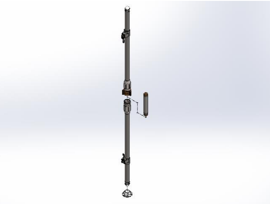
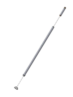
Figure 1 OptaSense Calibration tool and cal tool lite

The main differences between the Cal tool and the Cal tool lite are that the Cal tool is of a 2-piece titanium construction with a trigger mechanism at either end to hold the 3kg weight in place until the trigger is activated thus allowing the weight to fall to the other end of the tool and again be held by the trigger. This allows for quicker usage at the expense of adding more weight.

The Cal tool lite is a much simpler design in which one end of the aluminium tube is open and the weight is simply dropped into the tube and then impacts the stopper at the enclosed end. This tool has been designed to be shipped with project equipment and has a shorter life expectancy of the more robust calibration tool.

More information on both tools can be find on their respective data sheets. Calibration Tool and Calibration Tool lite.

A minimum of ten sequential drops are required at each calibrated location. The calibration point data is partnered with the collection of acoustic information to setup the detectors. This document describes the analysis of this acoustic data and has been designed to produce reliable and accurate results whilst also being as quick and easy to follow as possible. The number of calibration points required is dependent on the length of the asset. Every 1–2km for 40km would be sufficient with more or less being necessary as the asset length increased or decreased.

The results of your analysis should be recorded in the relevant Calibration Spreadsheet. One sheet should be completed for each OPS.

Calibration data should be collected both ON the asset (not necessarily the cable, the cable may be offset from the asset, but the asset to be protected is the key item and should be referred to primarily) and OFF the asset (e.g. at the ROW boundary or the agreed maximum desired extent for detections).

Importance of the Threat Profile

No calibration or detector configuration should be started in the absence of a completed threat profile from the customer – this is essential as this document should detail how the performance of detectors should vary along the right of the way – before commencing work in the field plan these activities around a deep discussion of the threat profile.

Use of the Calibration Tool energy limiter

The Calibration tool is provided with a “bung” to stop up each hole in the dead blow mass. The purpose of the hole is to let air pass through the mass and achieve a free fall – thus maximizing the impact energy. This is required towards the end of the sensing range to ensure that detections can be observed even in the hardest acoustic conditions, however closer to the IU this energy may be too great to accurately pin point the location and/or measure the acoustics. At the commencement of the calibration the bungs should be inserted and only when the acoustic reception becomes marginal should the bungs be removed.

note

If “Cal Tool Lite” is being used then there is no need for the energy limiter as the mass has been reduced accordingly.

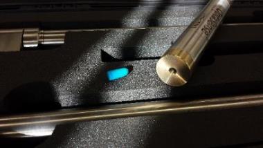
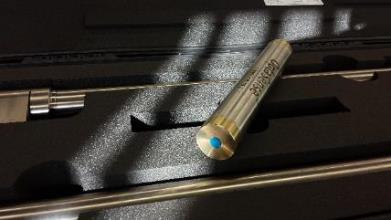
Figure 2: The Cal tool weight with the bung absent and fitted

Geo-refencing

With a working system, the following procedure should be followed to ensure that the fibre route is fully calibrated – this will result in the generation of calibration point data plus acoustic data for the setup of detectors (next chapter).

warning

The two activities should be carried out in parallel – failure to do will necessitate rework and revisits to site.

The purpose of the geographic calibration is to tie the optical distance to the linear asset distance. The Optical distance is normally significantly greater than the asset distance due to several factors:

• Fibre length over geographic distance (the optical distance of fibre in a cable is some percentage more than the linear distance). It is impossible for the optical distance to be shorter that the geographic distance.
• Fibre loops buried at junction points or in block valve stations (sometime hundreds of metres of extra fibre every 20km).
• Deviations of fibre route from asset route.

These need to be calibrated otherwise the system (which observes events in optical distance) will locate the events in the wrong location on the ground – which must be accurate for any valid response.

In most circumstances the client will have delivered routing data and kilometre marker (or equivalent) data and these will already have been input into the system. If the fibre route and KP’s are accurately represented on the map then the installer should follow Scheme 1 shown below.

Scheme 1:

• Locate a kilometre marker in the field
  • note the value
  • create an acoustic excitation
  • note the optical distance of the excitation
  • locate the kilometre marker position on the GUI
  • Create a calibration point at THIS position
  • Save the calibration point

If calibration marker points are NOT available as a pre-set but can be observed in the field the operator should follow Scheme 2 shown below.

Scheme 2:

• Locate a kilometre marker in the field
  • note the value
  • Note the GPS location
  • create an acoustic excitation
  • note the optical distance of the excitation
  • locate the GPS coordinates of the marker point on the GUI
  • Create a calibration point at THIS position
  • Save the calibration point

Finally, if no markers are present then the installer should follow Scheme 3 shown below:

Scheme 3:

• Locate known map features in the field (e.g. road crossings) and create acoustic excitation
  • Note the GPS location
  • note the optical distance of the excitation
  • Add a marker at GPS coordinates on the map, ensure that this marker is on or near the fibre
  • Create a calibration point at THIS position
  • Save the calibration point

Whichever method is being used, the actual actions to be taken are similar for the creation of the calibration point.

Entering Calibration Points

Using the methods outlined above, locate the desired position of the calibration points on the fibre (with a zoom in to be able to view the individual channels).

To display the fibre layer configuration, from the Configure menu, select Fibre Route.

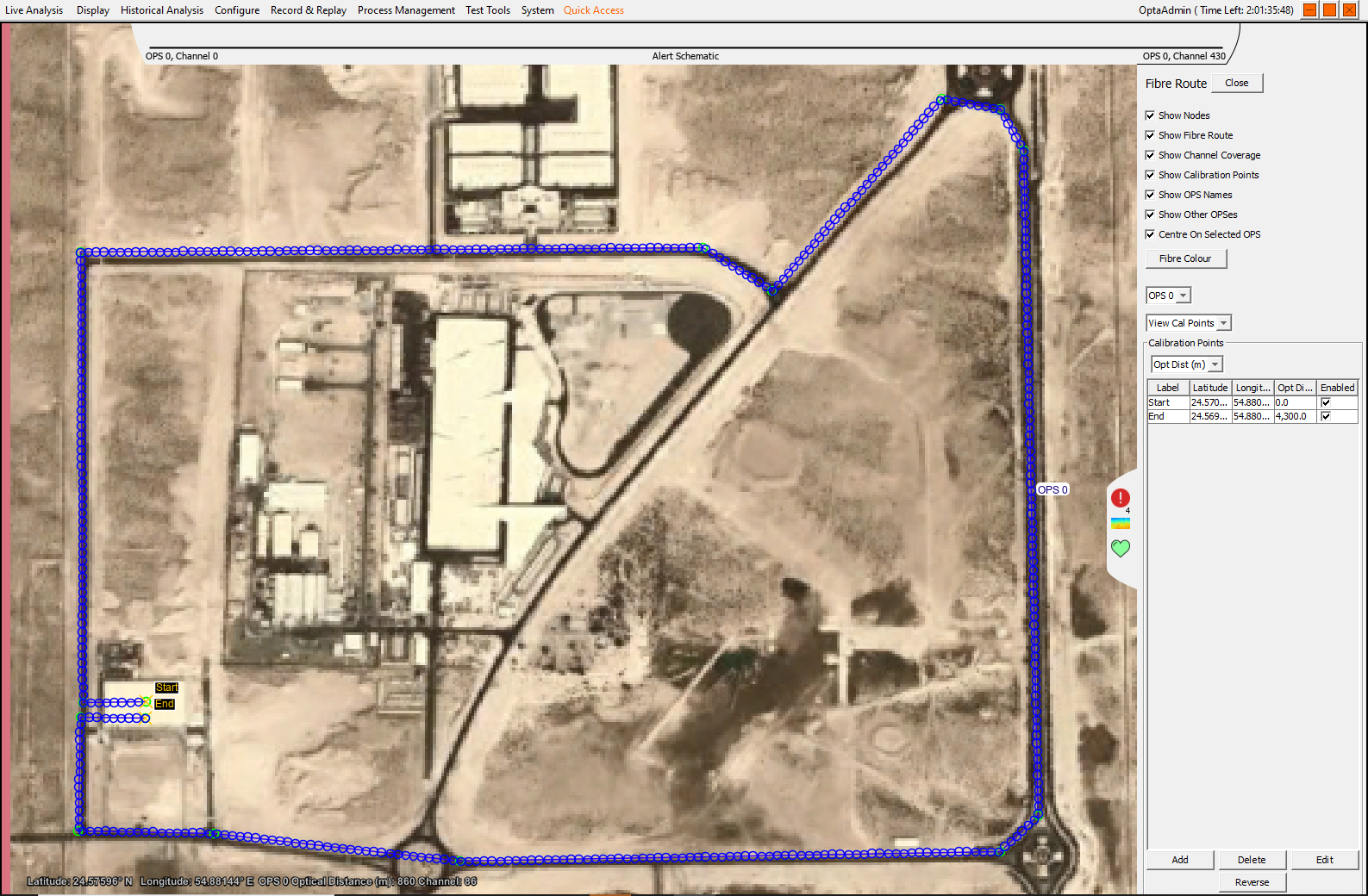
Figure 3: View of individual channels on route

Each channel is represented by an open circle of diameter equal to the channel length currently being used (e.g. 10m, 12.5m etc). The channels stay the same physical size no matter how the fibre route is calibrated (so for example, if a coil of fibre is represented a number of channels will be visible on top of each other). Equally if there is a significant gap between the circles then this suggests that the node routing or calibration position is wrong – it is telling you that there is more physical distance than there is fibre.

Locate the centre of the most appropriate channel and right click and select the Insert “Calibration Point option” from the pop-up menu. A dialogue box will then appear inviting you to enter the calibration data:

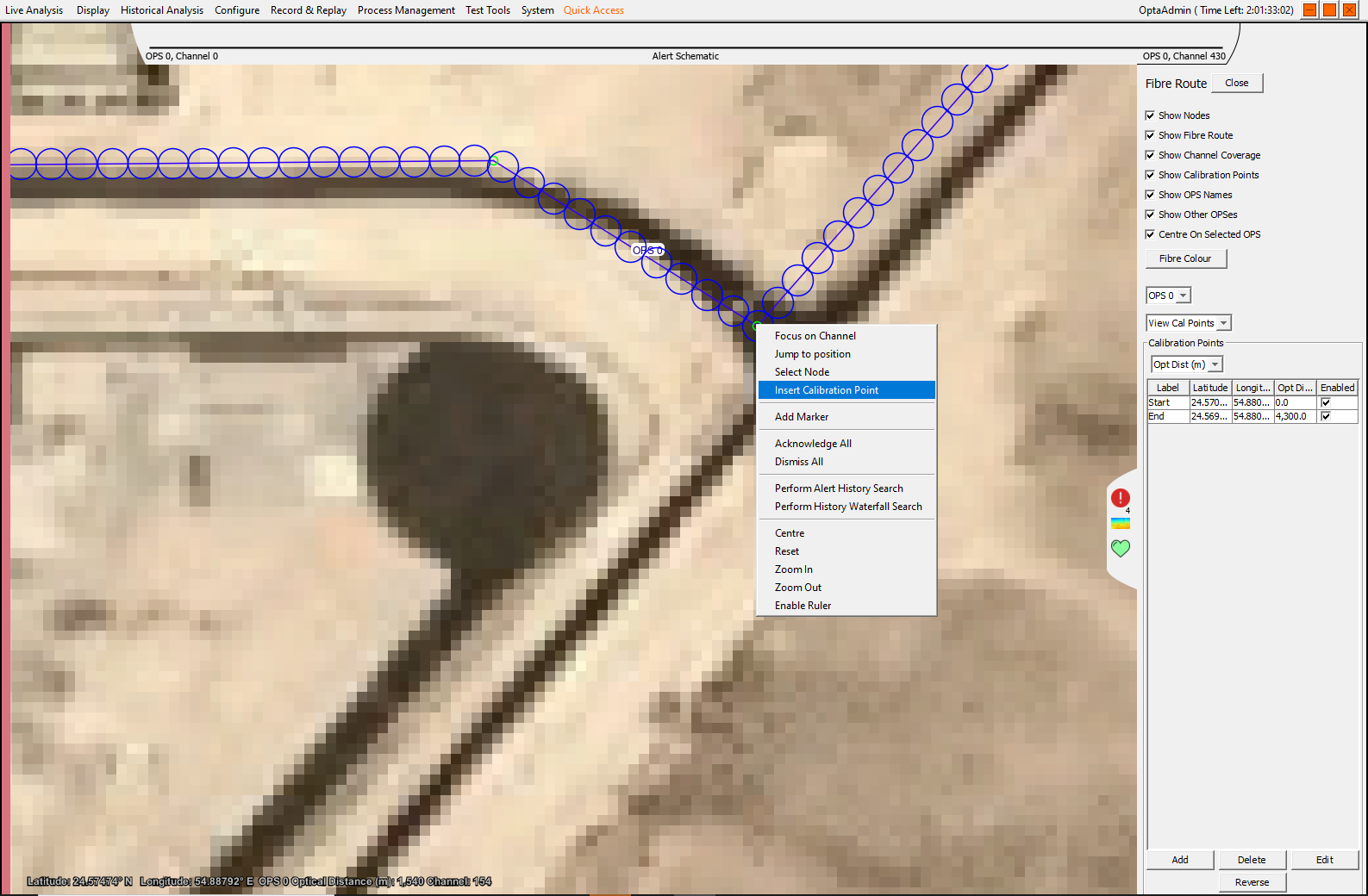
Figure 4: Entering calibration data

The Lat/Long will be picked from the location you have clicked on and so all that remains is to enter a label and the optical distance recorded from the Surveillance Waterfall display.

Collecting calibration data from the software

Once the calibration tool tests have been completed, the engineer can proceed to analysing the calibration data. This is a critical aspect of the calibration and greatly affects the downstream performance and ability to setup the detectors so must be followed carefully. Ideally the physical calibration field tests should be undertaken with an OptaSense calibration tool (where available).

Histogram Amplitude

1. Use the replay window to select and replay the relevant calibration data recording.
2. Use the Waterfall Histogram window to identify the channel with the highest amplitude signal from the calibration tool drops. If the signal is spread strongly across multiple channels, use the channel with the most consistent/highest amplitude values.

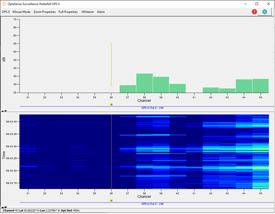
Figure 5: The histogram and surveillance waterfall

1. Use your mouse cursor to estimate the average amplitude of the calibration tool drops. To do this:
   1. Ensure that the waterfall update rates are set to 1:1
   2. Maximise the histogram window
   3. Zoom in on the channel (X) axis so that there are approximately 10 channels either side of the channel with the highest amplitude
   4. Zoom in on the amplitude (Y) axis so that the calibration tool drop signal is clear and uses most (~80%) of the display.

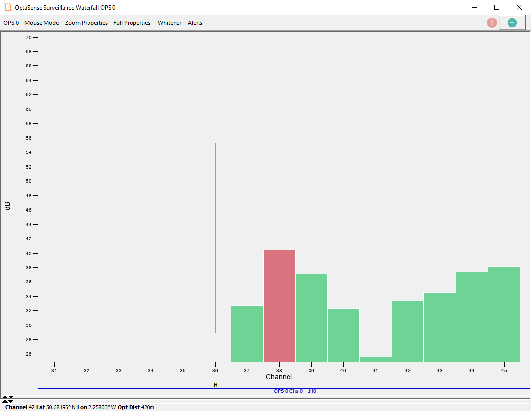
Figure 6: Use the window toggles (highlighted to the left) to maximise the histogram display.

1. Hover your mouse cursor at the peak of each drop, and gradually adjust to estimate the overall average amplitude across all drops. The amplitude should be averaged across all available calibration tool drops (this should be a minimum of 10 sequential drops)
2. Read the amplitude value off the status bar at the bottom of the window. Use this value as your Histogram Amplitude value for the data point / recording. The values do not have to be exact – the amplitude readings can typically be rounded to the nearest 100.

• Note: You are measuring the average amplitude; not the maximum amplitude. Care should be taken to appropriately adjust the cursor to represent the average. For this reason, calibration drops towards the end of the data recording will affect the overall average less than the initial signals.

**
**

Identifying the Max Frequency

1. Use the replay window to select and replay the relevant calibration data recording.
2. Use the Waterfall Histogram window to identify the channel with the highest amplitude signal from the calibration tool drops. If the signal is spread strongly across multiple channels, use the channel with the most consistent/highest amplitude values (this is very likely to be the channel used for the recording during the previous section).
3. Open an analysis window on the channel previously identified.

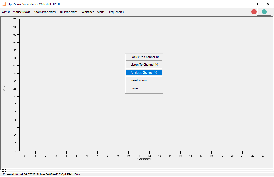
Figure 7: The ‘right click’ menu from the surveillance waterfall

1. In the FFT settings menu, select:
   1. Window size of 256
   2. Averaging of 1
   3. Overlap Percent of 50%
   4. Click Apply to ensure that the settings are saved
2. Maximise the spectrogram window by hovering the cursor over the left-hand-side of the spectrogram window, this area will then turn light grey (as indicated in figure 5, below). Click this toggle and drag & drop the spectrogram window out from the other analysis graphs. This window will then be separate from the others and can be maximised in the usual way.

• Note: The spectrogram window can also be separated by disabling the Time series, FFT and Periodogram display using the toggles on the right-hand side.

  

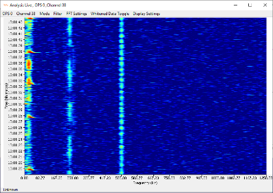
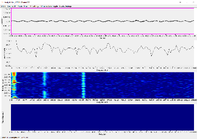
Figure 9: Separating the spectrogram display & then maximising the window can greatly assist the frequency analysis.

Go to the Spectrogram window from the Display Settings menu**,** replay the recording again and adjust the Min dB value until the background noise across the whole frequency range is minimal and just barely visible. This noise should appear as very faint light blue disperse & ‘speckled’ signals against a royal blue background, as follows:

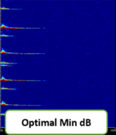
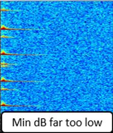
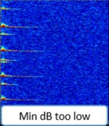
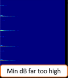
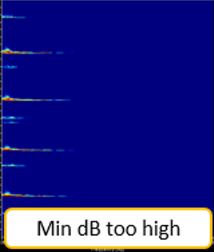
Figure 10: Evaluating the minimum dB value in the analysis window

1. Input the Max dB as 30dB higher than the Min dB value determined in the previous step. For instance, if the Min dB was found to be 5dB, input a Max dB value of 35.

• When setting the max dB, you may find that the visibility of the background noise increases. If this happens, slightly increase the Min dB value again in order to find the optimal point (as detailed in step 6). Once this has been fine-tuned, re-adjust the max dB to be 30dB higher.

  Your spectrogram will now be adjusted to provide the best Signal-to–Noise ratio (SNR) for the calibration recording.

1. Finally, replay the data recording once more, and use the spectrogram to estimate the maximum point across all the calibration drops at which the frequency response of the transients disappears into the noise floor. I.e. the maximum frequency at which the calibration signal is distinguishable from the noise floor, across all the calibration signal transients. This is not the average maximum; just the individual maximum detectable frequency out of all the tool drop signals.

   Hover your mouse above this point and note the frequency value on the status bar at the bottom. Use this value as your maximum frequency for this data point / recording (the values do not have to be exact - the frequency readings can be rounded to the nearest 10 Hz). Please see Annex A for some examples of this point.

• Note A: If you find that there are ‘gaps’ in the frequency range, you can effectively ‘ignore’ the gap and measure the maximum frequency as normal - refer to Annex B for some more guidance in this situation.
• Note B: If you need to change the channel you are analysing, it is more efficient to use the toggle in the ‘channel’ section of the analysis window (rather than opening a new window from scratch)

Maximum Frequency point examples

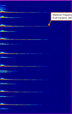
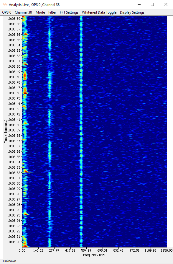
Figure 11: Evaluating the maximum frequency, example 1

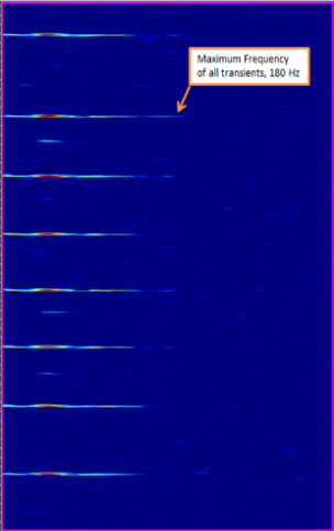
Figure 12: Evaluating the maximum frequency, example 2

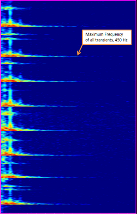
Figure 13: Evaluating the maximum frequency, example 3

Identifying the Transient Threshold & Transient Amplitude

In this section, the aim is to estimate initial manual digging detector settings by using the calibration data. Some prior knowledge of the detector is useful but is not required to complete the following steps.

1. Use the replay window to select and replay the relevant calibration data recording.
   NOTE: For this step, it is advisable to use the calibration recording with the maximum offset distance from the asset to begin with. Once these steps have been performed using this recording, you can use the recording above the asset confirm the suitability, as detailed in step 6. However, if no off-asset recording is available continue the below procedure using just the on-asset recording.
2. Use the Waterfall Histogram window to identify the channel with the highest amplitude signal from the calibration tool drops. If the signal is spread strongly across multiple channels, use the channel with the most consistent/highest amplitude values (this is very likely to be the channel used for the recording during the previous section).

• Open the Manual Digging Detector Control Window and zoom in so that there are approximately 20 channels either side of the channel centred on the calibration tool drop signal (to zoom in on the signal, simply click & drag on the graphical threshold display).

1. As a default starting point, ensure that the following parameters are set (refer to figure 4, page 5):
   1. Limit Update Rate in the Transients tab is set to 1 per second
   2. In the Transient Detector tab, use the following table to identify and set the minimum frequency. Select the column suitable for the recording offset, then select the row that represents the correct optical distance of the recording (use the closest rounded value – i.e. if the optical distance of the recording is 23km, use the 20km row).

Optical Distance (km) ˅	Maximum threat profile offset distance (m) >	0	5	10
0 10 20 30 40 50	60 Hz	50 Hz	40 Hz
	50 Hz	40 Hz	30 Hz
	40 Hz	30 Hz	20 Hz
	30 Hz	20 Hz	10 Hz
	20 Hz	10 Hz	5 Hz
	10 Hz	5 Hz	0 Hz

1. Maximum Frequency is set to the value found during the prior section (for the data point being used)
   1. Transient Threshold of 15
   2. Threshold (blue line) is set at 160

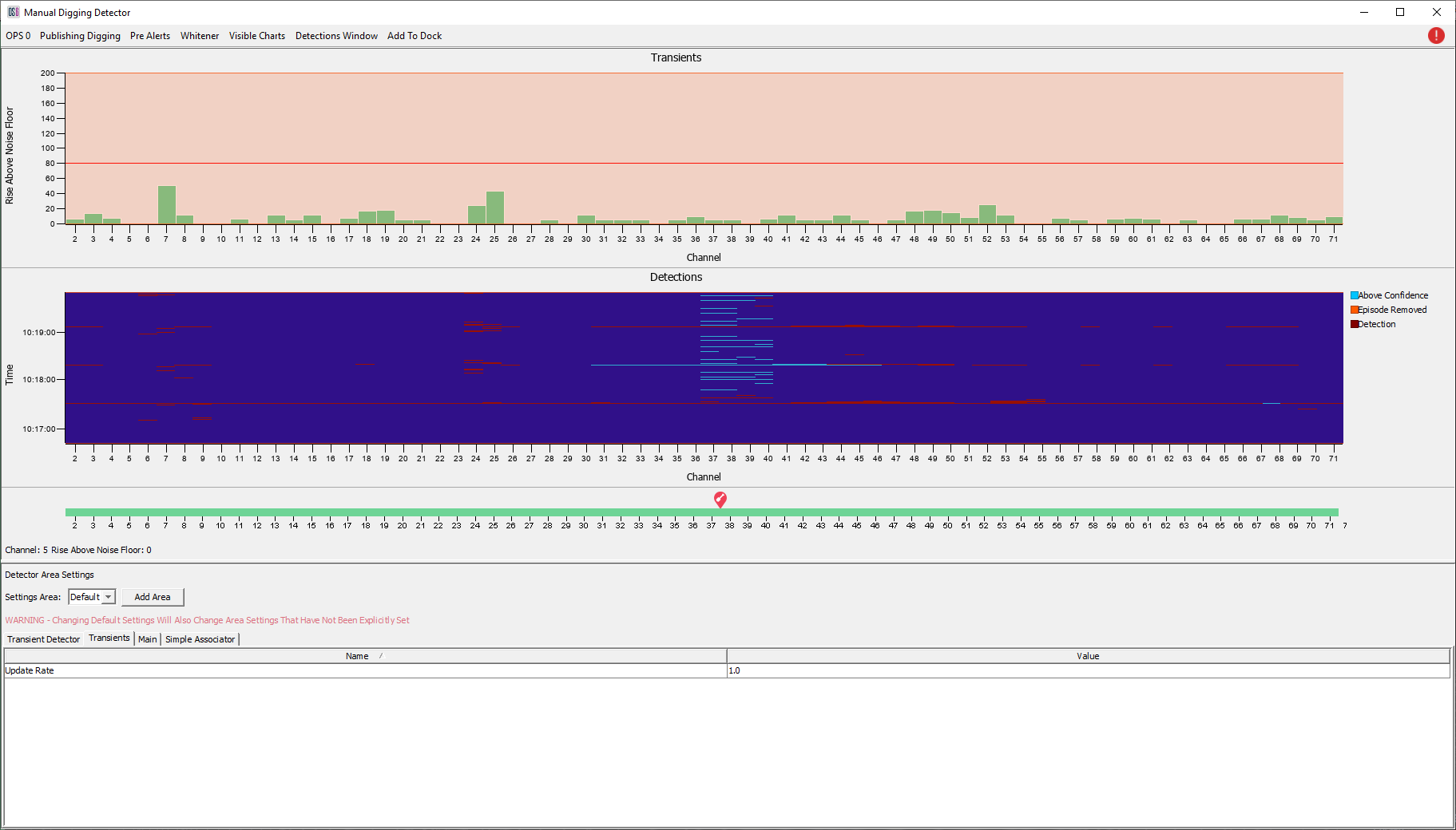
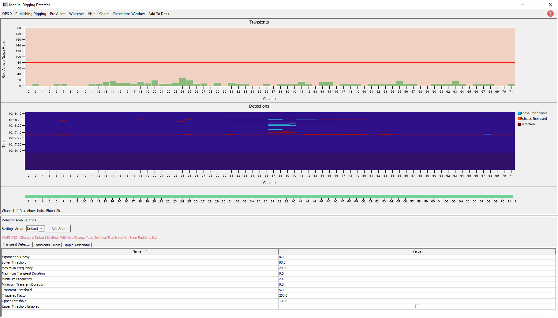
Figure 14: Configuring the Manual Digging Detector window for calibration analysis (refer to step 4)

1. Replay the recording and use the mouse to estimate the average amplitude of the calibration tool drop signals. Note this value, then proceed using the following logic:
   1. If the average amplitude is less than 160 (i.e. the blue line), lower the transient threshold (initially set to 15) by 1 and repeat step 5.
   2. If the average amplitude is greater than 160, record the value. Use this value as your threshold value for this data point / recording.

• Note: Do not go above a transient threshold value of 15. If the signal amplitude is consistently at 320 (i.e. the maximum value), then record a transient threshold of 15 and threshold of 320 as your value and continue as normal.

1. Record the transient threshold value used in step 5.

• Hint: At short optical distances (close to the IU) the initial transient threshold of 15 is likely to remain unchanged. However, this should progressively drop as the optical distance increases; particularly on longer or insensitive fibres.

1. Finally, replay the relevant on asset recording and confirm that the average amplitude is above 160. If not, repeat step 5 & 6 with this recording and note down the new transient threshold and amplitude threshold levels.

Evaluating Detector Areas

After the analysis of the calibration data is complete, these results can now be evaluated in order to inform and identify the Detector Areas to be used on the system. There are many different environmental factors that can affect the overall sensitivity of the system in any given area; fibre depth, fibre offset, fibre conduits or cable construction, the type of ground material (soil, arid ground, rock etc) moisture content of the ground material and obstructions (roads, rivers etc) to name but a few.

The main goal of the calibration analysis is to identify these areas of varying sensitivity, referred to in the OptaSense software and terminology as ‘Detector Areas’. As these detector areas represent areas of varying sensitivity, they also represent areas of different detector requirements. For instance, if a area is identified as being low sensitivity, then in general the detectors will need to be tuned to a high sensitivity to compensate. Thus, this is a critical outcome of the calibration procedure; once these detector areas are set they inform a vast amount of the system configuration and algorithm logic and approach.

Evaluating the analysis graphs

The calibration data details and results of the prior analysis should have been recorded in the relevant calibration spreadsheet. If not, enter them into a blank calibration spreadsheet now before proceeding. As data is entered into this spreadsheet, the graphs will automatically generate. These graphs can be viewed by selecting the relevant sheets within the spreadsheet.

• The ‘Charted by KP’ graphs show the analysis results on the Y axis, with the KP values on the X axis
• The ‘Charted by channel’ graphs show the analysis results on the Y axis, with the channel values on the X axis
• The ‘Separate Chart’ graphs show a variety of different graphs that can be used to supplement your evaluation of environmental zones to ensure confidence and reliability.
• Note: If all the results do not show (or they are displayed incorrectly), you may need to adjust the data range on the graphs. To do this, ‘right click’ a graph, choose ‘select data’ and then edit any data series so that it contains all the relevant results you are trying to plot.

Generally speaking, environmental zones should be defined by looking at all the graphs and identifying where the sensitivity of the system changes by a relatively large amount. This can be done in the following manner:

1. Use the ‘Charted by KP / channel’ sheets to evaluate the general trends of the signal. Providing the calibration data collection and analysis has been done correctly it relatively easy to identify areas of high, medium and low sensitivity.

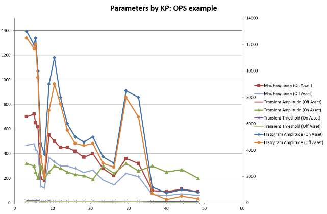
Figure 15: Example calibration sheet (charted by KP) with all parameters plotted

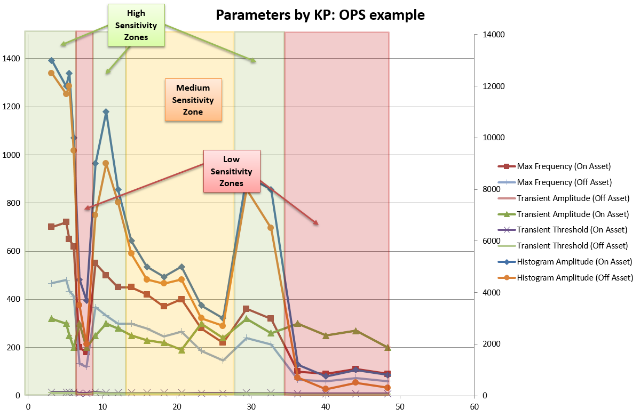
Figure 16: basic visual evaluation of the general trends can identify low, medium and high sensitivity zones

These low, medium & high areas can be used to get a good general idea of the environmental zone boundaries. In the above example, there would be 6 resultant environmental zones (approximately from KP 0 – 8, 8-9, 9-12, 12-28, 28-35 & 35- 48).

1. Once these rough boundaries have been identified, they can be verified / adjusted further by looking at the additional graphs – looking through the ‘on asset’ graphs and ‘off asset’ graphs will give a more detailed look at the trends and allow you to increase / decrease the size and placement of the zones appropriately. For instance, one of the ‘off asset’ zones may show that the area of low sensitivity is bigger than the overview graphs suggests; thus, it should be increased as necessary.

2. Finally, the ‘Separate Charts’ sheets should be consulted to verify by environmental zones. In particular, the ‘Transient Threshold vs Transient Amplitude’ graphs should be evaluated, as these distinctly show where the manual digging detectors have been varied throughout the calibration procedure.

   Boundaries where the Transient Threshold varies indicate the theoretical boundaries of environmental zones; these graphs should agree with your previous environmental zone estimates (from step 1 & 2). If not, then the detector areas can again be adjusted slightly, or potentially even another zone added if required.

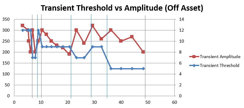
Figure 17: The Transient Threshold graphs indicate where different detectors / environmental zones are required (boundaries in the above graph are indicated by vertical blue lines). These should agree with your previous environmental zone analysis.

Once the detector areas have been evaluated, they can be configured into the system and the detector tuning process can begin.

The calibration sheets can provide valuable information throughout the installation and tuning process, so should be backed up and stored appropriately.

Anomalous conditions

Histogram Amplitude

Occasionally when measuring the histogram amplitude, you may encounter the uncommon situation where the outer channels from the calibration signal have a higher amplitude than the centre channels. As shown in the following image:

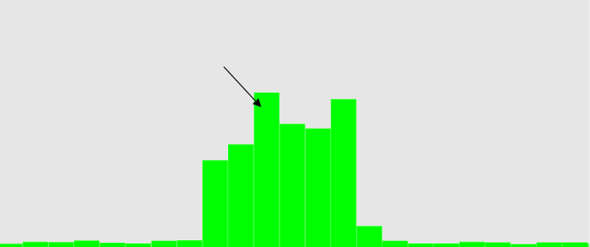
Figure 18: An uncommon calibration drop signal; the ‘outer’ channels are greater than the centre channels.

This can happen for a variety of reasons – either due to environmental or signal processing reasons. In this scenario, the procedure stays the same as before; replay the recording and identify the highest amplitude / most consistent channel and take the average amplitude of this channel using the cursor. In the above example this is marked with the black arrow.

Maximum Frequency Analysis

This part of the analysis asks you to evaluate the frequency range of the calibration tool drop signals. This is especially useful as it gives a good indication of the overall ground-to-fibre sensitivity levels in that environment. Part of this procedure involves changing the analysis window settings to optimally and appropriately measure the frequencies. A brief description of these settings is as follows:

1. Setting window size to 256 – this represents the default FFT window size for the third-party intrusion algorithms, and thus is the most appropriate value to use.
   1. Setting the averaging to 1 – this is a default and should not be changed
   2. Setting the overlap percent of 50% - this helps limit any ‘gaps’ in the frequency ranges – see below for some anomalous examples of this and how to proceed.

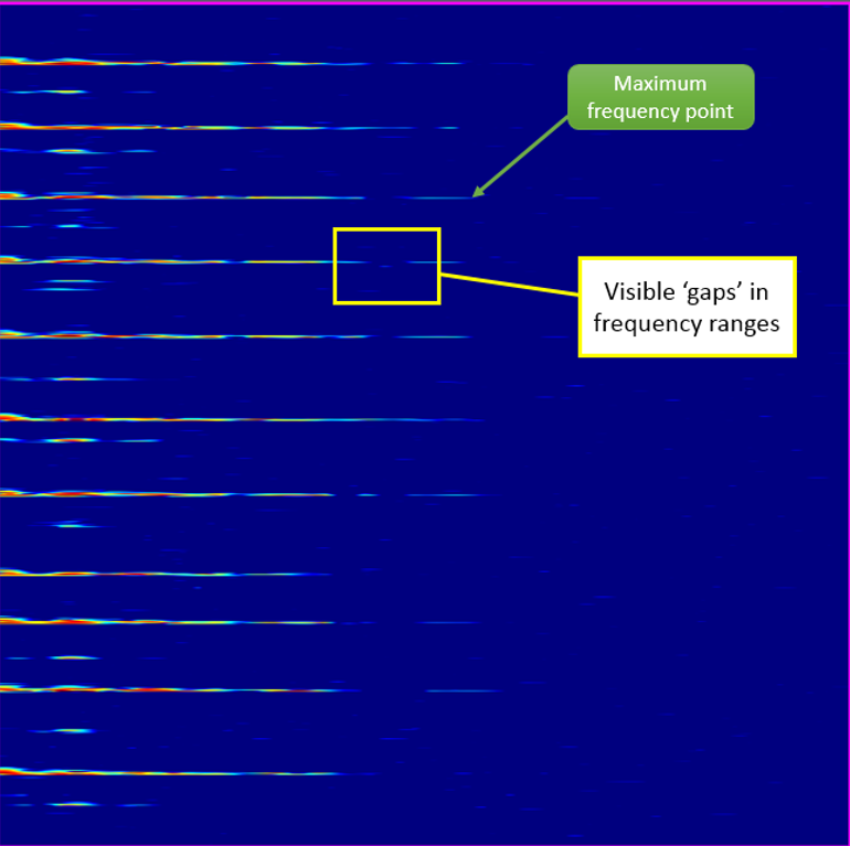
Figure 19: Occasionally visible ‘gaps’ in the calibration tool drop signals can be identified

As shown above, visible gaps in the frequency ranges of the calibration signals can sometimes occur. This is typically due to signal processing effects. Thus, when this happens you can effectively ‘ignore’ the gaps and measure the maximum frequency as normal – identify the maximum point at which the calibration tool signal is distinguishable from the background dark blue ‘noise’.

Transient Threshold / Transient Amplitude

Occasionally when measuring the transient amplitude, you may encounter the uncommon situation where the outer channels from the calibration signal have a higher amplitude than the centre channels. In this scenario, the procedure stays the same as before; replay the recording and identify the highest amplitude / most consistent channel and take the average amplitude of this channel using the cursor.